How the MSTmap algorithm works

This article describes the technical basis of the MSTmap algorithm (Wu et al. 2008) as it is implemented in ASMap. An understanding of its components is of practical value, since they correspond directly to arguments of the two construction functions.

Background

Genetic linkage maps consist of a set of polymorphic markers spanning the genome of a population derived from a cross between parental lines. They are used both to examine the genetic landscape of the population itself and, more commonly, to conduct gene–trait association studies such as quantitative trait loci (QTL) analysis or genomic selection. In QTL analysis in particular, the interpretation of significant genomic locations is improved when the markers have been assigned to chromosomal groups and optimally ordered within them.

Within the R environment (R Development Core Team 2014) a small number of packages perform linkage map construction. R/qtl (Broman and Wu 2014) provides an extensive set of tools for construction, exploration and manipulation across backcross, doubled haploid, intercrossed F2 and four-way populations, together with advanced recombinant inbred lines and populations arising from repeated backcrossing and selfing; it is documented at length by Broman and Sen (2009). R/onemap (Margarido and Mollinari 2014) offers comparable facilities for backcross, doubled haploid and recombinant inbred populations, and additionally for outcrossing populations.

Marker ordering in both packages proceeds in two stages. An initial order is obtained by a non-exhaustive method such as SERIATION (Buetow and Chakravarti 1987) or RECORD (Van Os et al. 2005); because such an order is not guaranteed to be optimal, it is then refined by exhaustively evaluating all permutations within a sliding marker window, a procedure known in the linkage mapping community as rippling. The computational cost of the second stage grows rapidly with the number of markers and the width of the window, and the procedure may require repetition before a stable order is reached.

ASMap was developed to avoid this two-stage structure (Taylor and Butler 2014; Taylor and Butler 2017). Its construction functions use the MSTmap algorithm (Wu et al. 2008), implemented as C++ source code and available separately from http://alumni.cs.ucr.edu/~yonghui/mstmap.html. The algorithm uses the minimum spanning tree of a graph (Cheriton and Tarjan 1976) both to cluster markers into linkage groups and to order markers within each group, in a single stage. It is applicable to backcross, doubled haploid and recombinant inbred populations; for the latter the level of self pollination may be specified, so that selfed F2, F3, $\ldots$ , Fn populations are accommodated, where $n$ denotes the level of selfing. Advanced recombinant inbred populations are treated as bi-parental for the purpose of construction.

Notation and objective functions

Following the notation of Wu et al. (2008), consider a doubled haploid population of $n$ individuals genotyped across a set of $t$ markers, in which each $(i,j)$ th entry of the $n \times t$ matrix $\boldsymbol{M}$ is either an $A$ or a $B$ , representing the two parental homozygotes. Let $\boldsymbol{P}_{jk}$ denote the probability of a recombination event between the markers $(\boldsymbol{m}_j, \boldsymbol{m}_k)$ , where $0 \leq \boldsymbol{P}_{jk} < 0.5$ . MSTmap admits two weight objective functions based on these recombination probabilities,

$\begin{aligned} w_p(j,k) &= \boldsymbol{P}_{jk} \qquad (1)\\ w_{ml}(j, k) &= -\bigl(\boldsymbol{P}_{jk}\log\,\boldsymbol{P}_{jk} + (1 - \boldsymbol{P}_{jk})\log(\,1 - \boldsymbol{P}_{jk})\bigr) \qquad (2) \end{aligned}$

In general $\boldsymbol{P}_{jk}$ is unknown and is replaced by the estimate $d_{jk}/n$ , where $d_{jk}$ is the Hamming distance between $\boldsymbol{m}_j$ and $\boldsymbol{m}_k$ , that is, the number of non-matching alleles between the two markers. This estimate is also the maximum likelihood estimate of $\boldsymbol{P}_{jk}$ for both weight functions.

These correspond to the objective.fun argument of the construction functions, "COUNT" selecting (1) and "ML" selecting (2).

Clustering markers into linkage groups

If markers $\boldsymbol{m}_j$ and $\boldsymbol{m}_k$ belong to different linkage groups then $\boldsymbol{P}_{jk} = 0.5$ , and the Hamming distance between them has the property $E(d_{jk}) = n/2$ . A thresholding mechanism for determining whether two markers belong to the same linkage group follows from Hoeffding’s inequality,

$\begin{aligned} P(d_{jk} < \delta) \leq \mbox{exp}(-2(n/2 - \delta)^2/n) \qquad (3) \end{aligned}$

for $\delta < 0.5$ . For a given $P(d_{jk} < \delta) = \epsilon$ and $n$ , the equation $-2(n/2 - \delta)^2/n = \mbox{log}\,\epsilon$ is solved to obtain an appropriate Hamming distance threshold $\hat{\delta}$ .

Wu et al. (2008) indicate that the choice of $\epsilon$ is not critical to the formation of linkage groups. The equation to be solved is, however, strongly dependent on the number of individuals in the population, and in practice the choice matters a great deal. The figure below shows, for a doubled haploid population, the profiles of $-\log_{10} \epsilon$ against population size for four threshold minimum cM distances $(25, 30, 35, 40)$ .

pValue(dist = c(25, 30, 35, 40), pop.size = 100:500, map.function = "kosambi")

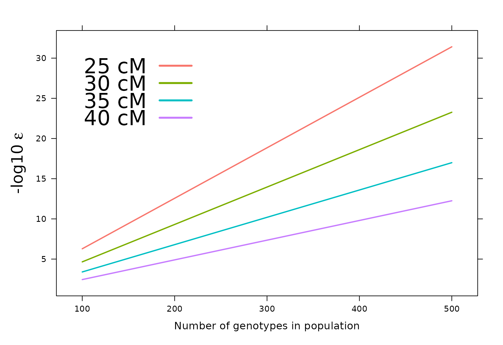
Negative log10 epsilon versus the number of genotypes in the population, for four threshold cM distances.

MSTmap adopts a default of $\epsilon = 0.00001$ , which is generally suitable for population sizes of $n \sim 150$ to $200$ . For larger populations the default becomes unsuitable. At $n = 350$ , for instance, the figure indicates that $\epsilon$ between $1.0e^{-12}$ and $1.0e^{-15}$ imposes a conservative minimum threshold of 30 to 35 cM before markers in different clusters are linked, whereas retaining the default lowers that threshold to approximately 45 cM, at which point distinct clusters of markers will appear linked.

The relationship between population size and p.value should be examined before construction is attempted. It is the argument that most often accounts for an implausible number of linkage groups.

Clustering itself proceeds by forming an edge-weighted undirected complete graph for $\boldsymbol{M}$ , in which the markers are vertices and the edge between any two markers $\boldsymbol{m}_j$ and $\boldsymbol{m}_k$ carries the pairwise Hamming distance $d_{jk}$ . Edges of weight greater than $\hat{\delta}$ are removed, and the remaining connected components partition the marker set into $r$ linkage groups, $\boldsymbol{M} = [\boldsymbol{M}_1,\ldots,\boldsymbol{M}_r]$ .

Ordering markers within a linkage group

Consider now the $n \times t$ matrix of markers $\boldsymbol{M}$ belonging to a single linkage group. Prior to ordering, the markers are binned into groups within which the pairwise distance between any two markers is zero. Markers within such a group exhibit no recombination between them and are said to co-locate at the same genomic position for the $n$ genotypes used in construction. A representative marker is selected from each bin to form the reduced $n \times t^*$ marker set $\boldsymbol{M}^*$ .

For the reduced matrix, consider the complete set of entries $(j, k) \in (1, \ldots, t^*)$ under either weight function (1) or (2). These may be viewed as the upper triangle of a symmetric weight matrix $\boldsymbol{W}$ , and equivalently as the connected edges of an undirected graph in which the markers are vertices. An order for the set $\boldsymbol{M}^*$ , also termed a travelling salesman path, is then obtained by visiting each marker once and summing the weights of the edges traversed. To find a path of minimum weight, MSTmap employs a minimum spanning tree algorithm (Cheriton and Tarjan 1976) such as that of Prim (1957).

Where the minimum weight path is unique, the minimum spanning tree gives the correct marker order. Where the data contain genotyping errors, or the number of individuals is small, the tree may not form a complete path and may instead contain markers or small sets of markers as nodes attached to it. In such cases MSTmap takes the longest path in the tree as a backbone and applies local optimisation techniques, among them K-opt, node relocation and block optimisation (see Wu et al. 2008), to improve upon the current path. The integration of these techniques is what permits ordering to be completed in a single stage.

Imputation of missing scores

Imputation of missing allele scores is performed by an EM type algorithm that is tightly integrated with the ordering procedure rather than applied as a preliminary step. The marker matrix $\boldsymbol{M}^*$ is converted to a matrix $\boldsymbol{A}$ whose entries express the probabilistic certainty of an allele being $A$ . For the $j$ th marker and $i$ th individual,

$\begin{aligned} \boldsymbol{A}(i,j) = \left\{\begin{array}{ll} 1 & \quad \mbox{if $\boldsymbol{M}^*(i,j)$ is the A allele}\\ 0 & \quad \mbox{if $\boldsymbol{M}^*(i,j)$ is the B allele}\\ \frac{(1 - \hat{\boldsymbol{P}}_{j - 1,j})(1 - \hat{\boldsymbol{P}}_{j,j+1})} {(1 - \hat{\boldsymbol{P}}_{j,j+1})(1 - \hat{\boldsymbol{P}}_{j,j+1}) + \hat{\boldsymbol{P}}_{j-1,j} \hat{\boldsymbol{P}}_{j,j+1}} & \quad \mbox{if $\boldsymbol{M}^*(i,j)$ is missing} \end{array}\right.\qquad (4) \end{aligned}$

where $\hat{\boldsymbol{P}}_{j,j-1}$ and $\hat{\boldsymbol{P}}_{j,j+1}$ are the estimated recombination fractions between the $(j-1)$ th and $j$ th markers and between the $j$ th and $(j+1)$ th markers respectively. The third expression is the posterior probability that the missing value at marker $j$ is the $A$ allele for genotype $i$ , given the current estimates.

The procedure begins by calculating pairwise normalised distances between all markers in $\boldsymbol{M}^*$ and deriving an initial weight matrix $\boldsymbol{W}$ . An undirected graph is formed from the markers and the upper triangular entries of $\boldsymbol{W}$ , and its minimum spanning tree establishes an initial order. For the current order at the $(j-1, j, j+1)$ th markers, the E-step updates the missing observation at marker $j$ through the estimates $\hat{\boldsymbol{P}}_{j-1,j} = \hat{d}_{j-1,j}/n$ and $\hat{\boldsymbol{P}}_{j,j+1} = \hat{d}_{j,j+1}/n$ in (4). The M-step then re-estimates the pairwise distances between all markers, where for the $j$ th and $k$ th marker

$\begin{aligned} \hat{d}_{jk} = \sum_{i = 1}^{t^*}\boldsymbol{A}(i,j)(1 - \boldsymbol{A}(i, k)) + \boldsymbol{A}(i,k)(1 - \boldsymbol{A}(i, j)) \qquad (5) \end{aligned}$

and $\boldsymbol{W}$ is recalculated. A new undirected graph is formed, a new order derived from its minimum spanning tree, and the procedure repeated to convergence. Several iterations are generally required, though the computation remains expedient; computation time increases with the number of missing values.

This procedure underlies the mvest.bc argument, which is discussed further in Notes on the MSTmap algorithm.

Detection of genotyping errors

The algorithm can additionally detect and remove probable genotyping errors, again as part of the ordering procedure. A weighted average of nearby markers determines the expected state of an allele; for individual $i$ and marker $j$ ,

$\begin{aligned} \mbox{E}[\boldsymbol{A}(i, j)] = \sum_{j \neq k}d_{j,k}^{-2}\boldsymbol{A}(i,k)\bigg/\sum_{j \neq k}d_{j,k}^{-2} \qquad (6) \end{aligned}$

where the weights are the inverse squared distances from marker $j$ to its neighbours. Only a small set of nearby markers is used at each iteration, and an observed allele is regarded as suspicious when $|\mbox{E}[\boldsymbol{A}(i, j)] - \boldsymbol{A}(i, j)| > 0.75$ . A suspicious observation is set to missing and imputed by the EM algorithm described above.

Removing a suspicious allele reduces the number of recombinations between the marker concerned and its neighbours. This has a direct effect on the estimated genetic distances and hence on the overall length of the linkage group, and the option should therefore be used deliberately rather than routinely.

This is the basis of the detectBadData argument, examined in Notes on the MSTmap algorithm.

References

Broman, K. W, and S Sen. 2009. A Guide to QTL Mapping with R/qtl. Springer-Verlag.

Broman, K. W, and H Wu. 2014. qtl: Tools for Analyzing QTL Experiments. https://CRAN.R-project.org/package=qtl.

Buetow, K. H, and A Chakravarti. 1987. “Multipoint gene mapping using seriation. 1 General methods.” American Journal of Human Genetics 41: 180–88.

Cheriton, D., and R. E. Tarjan. 1976. “Finding Minimum Spanning Trees.” SIAM Journal on Computing 5 (4): 724–42. https://doi.org/10.1137/0205051.

Margarido, G, and M Mollinari. 2014. onemap: Software for constructing genetic maps in experimental crosses: full-sib, RILs, F2 and backcrosses. https://CRAN.R-project.org/package=onemap.

Prim, R. C. 1957. “Shortest Connection Networks and Some Generalizations.” Bell System Technical Journal 36: 1389–401.

R Development Core Team. 2014. R: A Language and Environment for Statistical Computing. R Foundation for Statistical Computing. http://www.R-project.org.

Taylor, J. D, and D Butler. 2014. ASMap: An (A)ccurate and (S)peedy linkage map construction package for inbred populations that uses the extremely efficient MSTmap algorithm. http://www.CRAN.R-project.org/src/contrib/Archive/ASMap/.

Taylor, Julian, and David Butler. 2017. “R Package ASMap: Efficient Genetic Linkage Map Construction and Diagnosis.” Journal of Statistical Software 79 (6): 1–29. https://doi.org/10.18637/jss.v079.i06.

Van Os, Hans, Piet Stam, Richard Visser, and Herman Van Eck. 2005. “RECORD: A Novel Method for Ordering Loci on a Genetic Linkage Map.” TAG Theoretical and Applied Genetics 112: 30–40. http://dx.doi.org/10.1007/s00122-005-0097-x.

Wu, Yonghui, Prasanna R. Bhat, Timothy J. Close, and Stefano Lonardi. 2008. “Efficient and Accurate Construction of Genetic Linkage Maps from the Minimum Spanning Tree of a Graph.” PLoS Genetics 4 (10). https://doi.org/10.1371/journal.pgen.1000212.