Notes on the MSTmap algorithm

These notes refer to objects built in Worked example I. The code below rebuilds them.

These notes concern aspects of the MSTmap algorithm, and of the arguments supplied to the construction functions, that emerge only from detailed use. Each has the same practical consequence: apparently inflated genetic distances.

Inflation of genetic distances

There are circumstances in which the algorithm produces inflated genetic distances. This is most pronounced when the map being constructed contains genotypes with many missing values, since the constructed map will then contain runs of missing values for those genotypes.

plotMissing(mapBC4)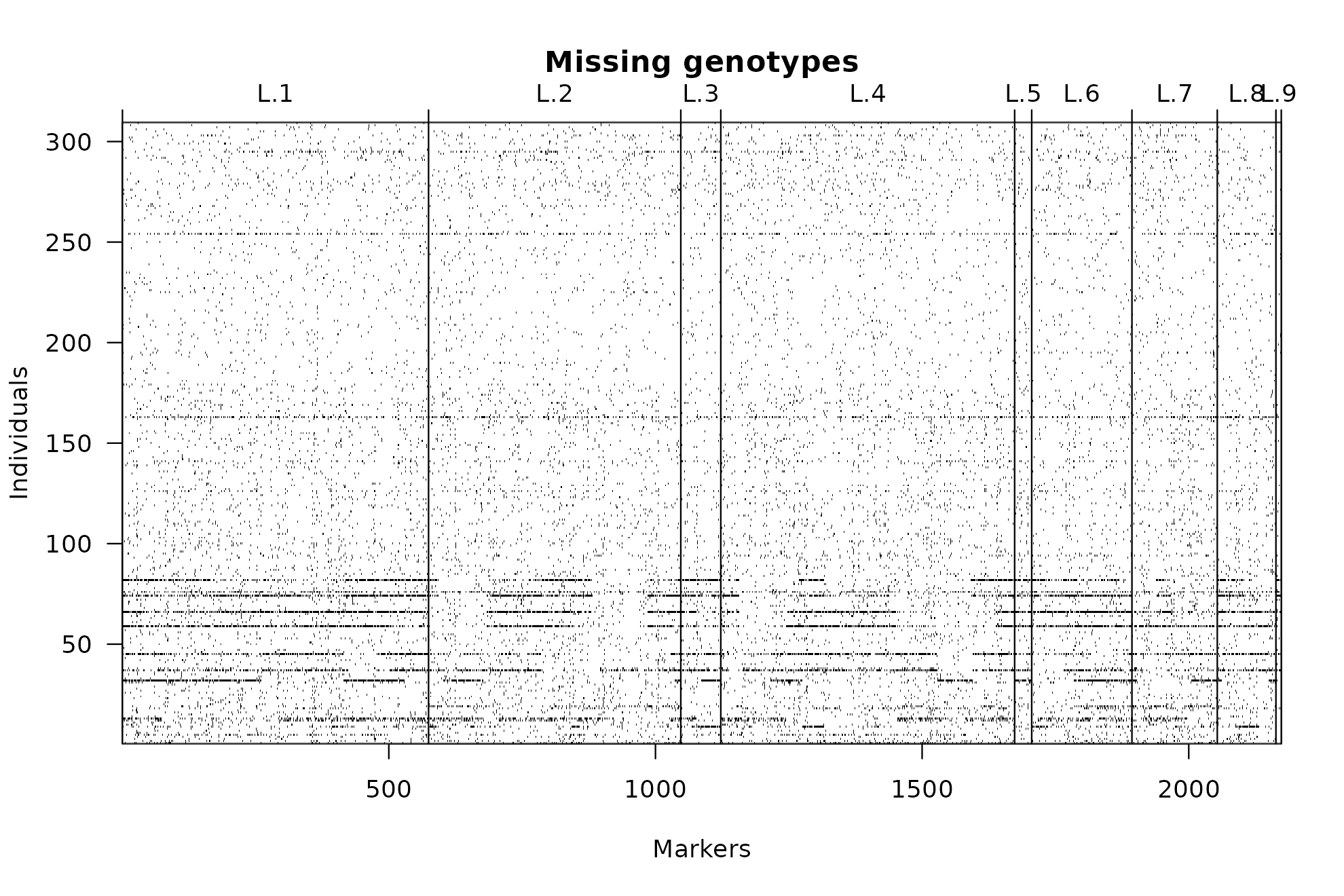

Missing allele scores for the constructed map mapBC4.

The dark lines show the phenomenon in the initial map mapBC4. Seven of these genotypes were eventually removed for excessive recombination across the genome, but their missing value structure contributed substantially to the inflated lengths of the linkage groups in its own right.

The mechanism is most easily shown by reconstructing the map with return.imputed = TRUE, which adds the imputed marker probability matrix to the returned object.

mapBC4i <- mstmap(mapBC3, bychr = FALSE, trace = FALSE, dist.fun = "kosambi",
                  p.value = 1e-12, return.imputed = TRUE)

Number of linkage groups: 9
The size of the linkage groups are: 574 473 75  551 32  188 160 110 10  
The number of bins in each linkage group: 182   204 31  191 18  91  73  60  6   

mapBC4i$geno[[1]]$map[1:14]

  mark246   mark986  mark1452  mark2266   mark391   mark426   mark670  mark1220 
0.0000000 0.0000000 0.0000000 0.0000000 0.7641466 0.7641466 0.7641466 0.7641466 
 mark1789  mark2193  mark2269  mark2382  mark2579  mark2934 
0.7641466 0.7641466 0.7641466 0.7641466 0.7641466 0.7641466 

mapBC4i$imputed.geno[[1]]$map[1:5]

  mark246   mark391   mark284   mark157  mark1990 
0.0000000 0.7641466 1.5507414 2.3555151 3.4031908 

Consider the markers on L.1. The first 14 markers contain the first two co-locating sets and are calculated to lie 0.76 cM apart. The imputed map is a reduced form containing all unique markers together with one member of each co-locating set; mark246 and mark391 are the members chosen for the first two sets. The number of observed allele pairs between the two markers, and the number of observed recombinations across those pairs, may be counted directly.

len <- apply(mapBC4$geno[[1]]$data[, c(1, 5)], 1, function(el)
             length(el[!is.na(el)]))
length(len[len > 1])

[1] 281

bca <- apply(mapBC4i$geno[[1]]$data[, c(1, 5)], 1, function(el) {
    el <- el[!is.na(el)]
    sum(abs(diff(el)))
})
bca[bca > 0]

BC004 
    1 

A single genuine recombination among 281 observed pairs implies a distance of 0.35 cM, well short of the 0.76 cM reported. The shortfall is explained by the imputed marker probabilities for the first five markers of the seven genotypes carrying excessive missing values.

mapBC4i$imputed.geno[[1]]$data[pg$xo.lambda, 1:5]

           mark246     mark391     mark284    mark157    mark1990
BC009 1.000000e+00 1.000000000 1.000000000 1.00000000 1.000000000
BC013 1.026860e-03 0.000000000 0.002317796 0.00000000 0.003386561
BC032 1.000000e+00 0.735586234 0.672130843 0.60287457 0.639670176
BC061 5.363308e-01 0.552323021 0.539409197 0.54183522 1.000000000
BC069 0.000000e+00 0.008689148 0.000000000 0.02198752 0.035294621
BC077 3.478224e-07 0.000000000 0.000000000 0.00000000 0.000000000
BC085 9.095952e-01 0.955278155 1.000000000 0.90765213 0.881923903

Genotype BC061 has an extended run of missing values across the first four co-located sets. Under the distance formula in the M-step of the EM algorithm, given as equation (5) in How the MSTmap algorithm works, the estimated probabilities for its two missing scores in the first two markers contribute a further half recombination, or approximately 0.15 cM, to the distance between them. BC061 contributes similarly between the second and third sets and between the third and fourth, because the imputed probabilities remain close to 0.5 throughout the run. Where several genotypes carry such runs, these small contributions accumulate quickly and the linkage groups appear inflated.

Two remedies are available. The first is to remove the offending genotypes, irrespective of their value elsewhere in the map. The second, less obvious, is to re-estimate the distances with quickEst(); because that function imputes missing values with actual allele calls, it avoids the uncertain probabilities from which MSTmap forms its distances.

mapBC4e <- quickEst(mapBC4)
chrlen(mapBC4)

       L.1        L.2        L.3        L.4        L.5        L.6        L.7 
304.910957 266.240647  78.982131 252.281760  33.226962 233.485952 153.315888 
       L.8        L.9 
106.290403   6.657526 

chrlen(mapBC4e)

       L.1        L.2        L.3        L.4        L.5        L.6        L.7 
213.056491 201.340804  63.404825 187.741586  26.574889 189.370258 132.623157 
       L.8        L.9 
 77.211705   2.912879 

The reduction is substantial: in excess of 80 cM for L.1, and over 60 cM for both L.2 and L.4.

Where a map has been constructed from genotypes carrying many missing values, the missing value structure of the resulting object should be examined. If runs of missing values are present the linkage groups are most likely inflated, and the distances should be checked with quickEst().

The argument mvest.bc

Inflation of this kind can be made considerably worse by injudicious use of mvest.bc.

The reason lies in how co-segregating markers are determined. In the initial stages of the algorithm two markers are held to be co-located if their pairwise distance is zero, that distance being computed only from allele pairs observed in both markers. A representative is chosen from each co-locating set, the remainder set aside with a record of their link to it, and the map constructed from the representatives alone. This is the behaviour under mvest.bc = FALSE.

Under mvest.bc = TRUE, missing allele calls are instead assigned a probability of 0.5 of being an A allele before clustering takes place. This has the evident advantage of involving the complete set of genotypes in the pairwise calculations. It has a less evident consequence: for any two markers with some proportion of unobserved allele pairs, the pairwise distance becomes non-zero, and the markers are therefore not judged co-located. A larger set of markers consequently enters construction, with the original missing calls imputed repeatedly as part of marker ordering. Where missing values are concentrated in a subset of genotypes, the cumulative distances between adjacent markers increase quickly.

mapBC4a <- mstmap(mapBC3, bychr = FALSE, trace = FALSE, dist.fun = "kosambi",
                  p.value = 1e-12, mvest.bc = TRUE)

Number of linkage groups: 9
The size of the linkage groups are: 574 473 75  551 32  188 160 110 10  
The number of bins in each linkage group: 566   412 75  496 32  188 135 109 10  

nmar(mapBC4)

L.1 L.2 L.3 L.4 L.5 L.6 L.7 L.8 L.9 
574 473  75 551  32 188 160 110  10 

Clustering yields an identical number of linkage groups containing the same markers. The number of uniquely located markers within each group, however, increases considerably, and with it the length of each group.

sapply(mapBC4a$geno, function(el) length(unique(round(el$map, 4)))) -
  sapply(mapBC4$geno, function(el) length(unique(round(el$map, 4))))

L.1 L.2 L.3 L.4 L.5 L.6 L.7 L.8 L.9 
384 208  44 305  14  97  62  49   4 

chrlen(mapBC4a)

       L.1        L.2        L.3        L.4        L.5        L.6        L.7 
498.063994 340.716640  96.513164 356.269346  41.016980 275.675999 164.254019 
       L.8        L.9 
123.280455   6.952472 

The remedy is again quickEst().

mapBC4b <- quickEst(mapBC4a)
chrlen(mapBC4b)

      L.1       L.2       L.3       L.4       L.5       L.6       L.7       L.8 
207.88659 199.40969  62.42760 184.52014  25.92514 187.42973 132.71937  75.91499 
      L.9 
  2.58925 

The argument detectBadData

The preceding sections concern inflation arising from missing values. Where missing values are not the cause and distances remain inflated, the explanation is most likely an increased recombination rate among some or all genotypes, which is readily checked with statGen() or profileGen() once an initial map exists.

An increased rate confined to a few genotypes is dealt with by removing them. A general inflation across many or all genotypes is more awkward, and suggests genotyping errors introduced during the physical process of obtaining the allele calls.

Setting detectBadData = TRUE instructs MSTmap to identify suspiciously called alleles, by the criterion given as equation (6) in How the MSTmap algorithm works. Suspicious calls are set to missing and imputed by the EM algorithm, which reduces the number of recombinations between adjacent markers and may reduce both those distances and the overall linkage group lengths substantially.

The behaviour is illustrated by introducing simulated genotyping errors into the final map mapBC, switching individual allele calls at random within each linkage group.

mapBCd <- mapBC
mapBCd$geno <- lapply(mapBCd$geno, function(el) {
    ns <- sample(1:ncol(el$data), ncol(el$data) / 2, replace = TRUE)
    ns <- cbind(sample(1:nrow(el$data), ncol(el$data) / 2, replace = TRUE), ns)
    el$data[ns] <- abs(1 - el$data[ns])
    el$data[el$data == 0] <- 2
    el
})
mapBCd <- quickEst(mapBCd)
chrlen(mapBCd)

     L.1      L.2      L.3      L.4      L.5      L.6      L.7 
262.7372 265.0427 169.6948 252.3984 223.7460 168.1366 153.2918 

quickEst() does not disregard the introduced errors, and the linkage groups are correspondingly inflated.

mapBCda <- mstmap(mapBCd, bychr = TRUE, trace = FALSE, dist.fun = "kosambi",
                  p.value = 1e-12, detectBadData = TRUE)

Number of linkage groups: 1
The size of the linkage groups are: 681 
The number of bins in each linkage group: 219   
Number of linkage groups: 1
The size of the linkage groups are: 593 
The number of bins in each linkage group: 229   
Number of linkage groups: 1
The size of the linkage groups are: 335 
The number of bins in each linkage group: 100   
Number of linkage groups: 1
The size of the linkage groups are: 679 
The number of bins in each linkage group: 217   
Number of linkage groups: 1
The size of the linkage groups are: 233 
The number of bins in each linkage group: 110   
Number of linkage groups: 1
The size of the linkage groups are: 279 
The number of bins in each linkage group: 100   
Number of linkage groups: 1
The size of the linkage groups are: 219 
The number of bins in each linkage group: 112   

chrlen(mapBCda)

     L.1      L.2      L.3      L.4      L.5      L.6      L.7 
228.9131 224.6887 141.4048 205.6216 196.4040 142.0062 137.3560 

Detecting and disregarding the errors during marker ordering returns the linkage groups to lengths comparable with those of the final map mapBC.

detectBadData alters the data on which distances are based, and will reduce linkage group lengths whether or not genotyping errors are truly present. It should be applied deliberately, once other explanations for inflation have been excluded, rather than as a routine setting.

Further reading

• How the MSTmap algorithm works — the imputation and error detection procedures these arguments control
• Manipulating linkage maps — quickEst() in detail
• Worked example I — the map these notes refer to

References

Taylor, Julian, and David Butler. 2017. “R Package ASMap: Efficient Genetic Linkage Map Construction and Diagnosis.” Journal of Statistical Software 79 (6): 1–29. https://doi.org/10.18637/jss.v079.i06.