Worked example II: refinement

This article continues the worked example. The code below rebuilds the map as it stood at the end of Worked example I.

Reintroducing the markers set aside

The markers placed aside during pre-construction are now returned to the constructed map, which is then re-diagnosed. The 515 markers carrying between 10% and 20% missing values, held in the "missing" element, are restored first.

mapBC6 <- pushCross(mapBC6, type = "missing",
                    pars = list(miss.thresh = 0.22, max.rf = 0.3))

A threshold of miss.thresh = 0.22 ensures that all markers below that proportion are restored. Recall that this mechanism assigns markers to the most suitable linkage group but does not reconstruct the map.

It is worth re-examining the heat map at this point to establish whether the restoration has been successful. The display is confined to linkage groups L.3, L.5, L.8 and L.9, to determine whether the additional markers bear on the possible merging of those groups.

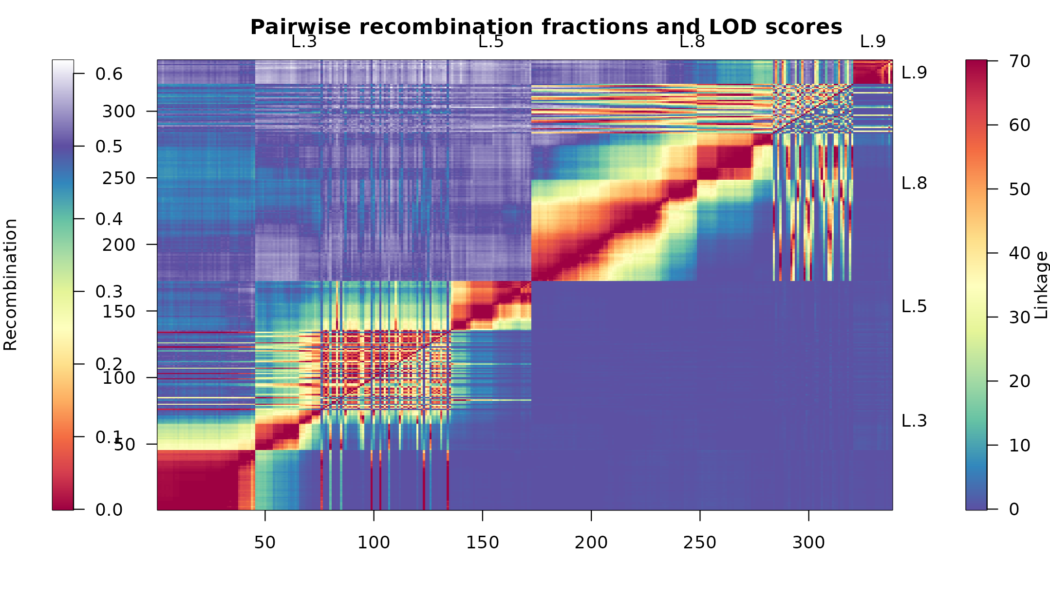
heatMap(mapBC6, chr = c("L.3", "L.5", "L.8", "L.9"), lmax = 70)

Heat map of linkage groups L.3, L.5, L.8 and L.9 of mapBC6.

Genuine linkage is evident between L.3 and L.5, and between L.8 and L.9. These two pairs are merged with mergeCross() and the groups renamed, giving the seven linkage groups expected for the barley genome.

mapBC6 <- mergeCross(mapBC6, merge = list("L.3" = c("L.3", "L.5"),
                                          "L.8" = c("L.8", "L.9")))
names(mapBC6$geno) <- paste("L.", 1:7, sep = "")
mapBC7 <- mstmap(mapBC6, bychr = TRUE, trace = FALSE, dist.fun = "kosambi",
                 p.value = 2)

Number of linkage groups: 1
The size of the linkage groups are: 680 
The number of bins in each linkage group: 196   
Number of linkage groups: 1
The size of the linkage groups are: 570 
The number of bins in each linkage group: 213   
Number of linkage groups: 1
The size of the linkage groups are: 172 
The number of bins in each linkage group: 72    
Number of linkage groups: 1
The size of the linkage groups are: 673 
The number of bins in each linkage group: 205   
Number of linkage groups: 1
The size of the linkage groups are: 233 
The number of bins in each linkage group: 99    
Number of linkage groups: 1
The size of the linkage groups are: 192 
The number of bins in each linkage group: 83    
Number of linkage groups: 1
The size of the linkage groups are: 166 
The number of bins in each linkage group: 84

chrlen(mapBC7)

     L.1      L.2      L.3      L.4      L.5      L.6      L.7 
242.4104 233.1945 162.6205 224.1773 201.1503 147.7669 159.5308

Since the optimal number of linkage groups has been established, reconstruction proceeds by linkage group alone, through p.value = 2. Anchoring is unnecessary here, as the orientation of the groups has not yet been formally determined.

The lengths of L.1, L.2 and L.4 are somewhat elevated, indicating excessive recombination across those groups. The cause is apparent from the genotype profiles.

pg1 <- profileGen(mapBC7, bychr = FALSE, stat.type = c("xo", "dxo", "miss"),
                  id = "Genotype", xo.lambda = 14, layout = c(1, 3), lty = 2,
                  cex = 0.7)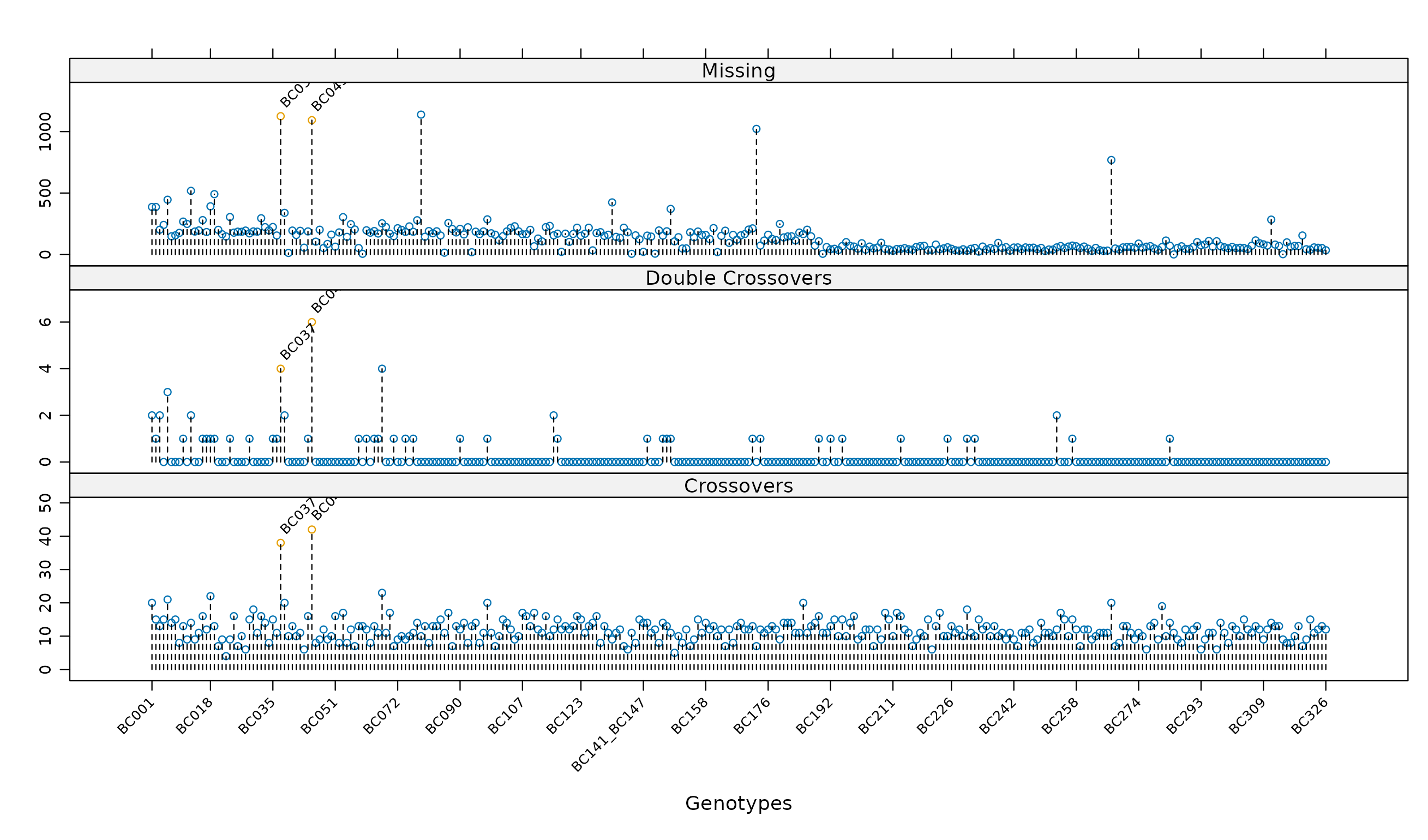

For individual genotypes, the number of recombinations, double recombinations and missing values for mapBC7.

Introducing the markers with 10 to 20% missing values has exposed two further problematic lines carrying a high proportion of missing values across the genome. These are removed and the map reconstructed.

mapBC8 <- subsetCross(mapBC7, ind = !pg1$xo.lambda)
mapBC9 <- mstmap(mapBC8, bychr = TRUE, dist.fun = "kosambi", trace = FALSE,
                 p.value = 2)

Number of linkage groups: 1
The size of the linkage groups are: 680 
The number of bins in each linkage group: 192   
Number of linkage groups: 1
The size of the linkage groups are: 570 
The number of bins in each linkage group: 210   
Number of linkage groups: 1
The size of the linkage groups are: 172 
The number of bins in each linkage group: 70    
Number of linkage groups: 1
The size of the linkage groups are: 673 
The number of bins in each linkage group: 203   
Number of linkage groups: 1
The size of the linkage groups are: 233 
The number of bins in each linkage group: 98    
Number of linkage groups: 1
The size of the linkage groups are: 192 
The number of bins in each linkage group: 83    
Number of linkage groups: 1
The size of the linkage groups are: 166 
The number of bins in each linkage group: 83

chrlen(mapBC9)

     L.1      L.2      L.3      L.4      L.5      L.6      L.7 
225.7900 223.3063 157.0592 206.4801 194.3003 145.7554 149.2467

Removing two lines does not affect the number of linkage groups, so reconstruction is again by linkage group only. The lengths of most groups are now appreciably reduced.

Restoring the distorted markers

profileMark(mapBC9, stat.type = c("seg.dist", "prop"), layout = c(1, 3),
            type = "l")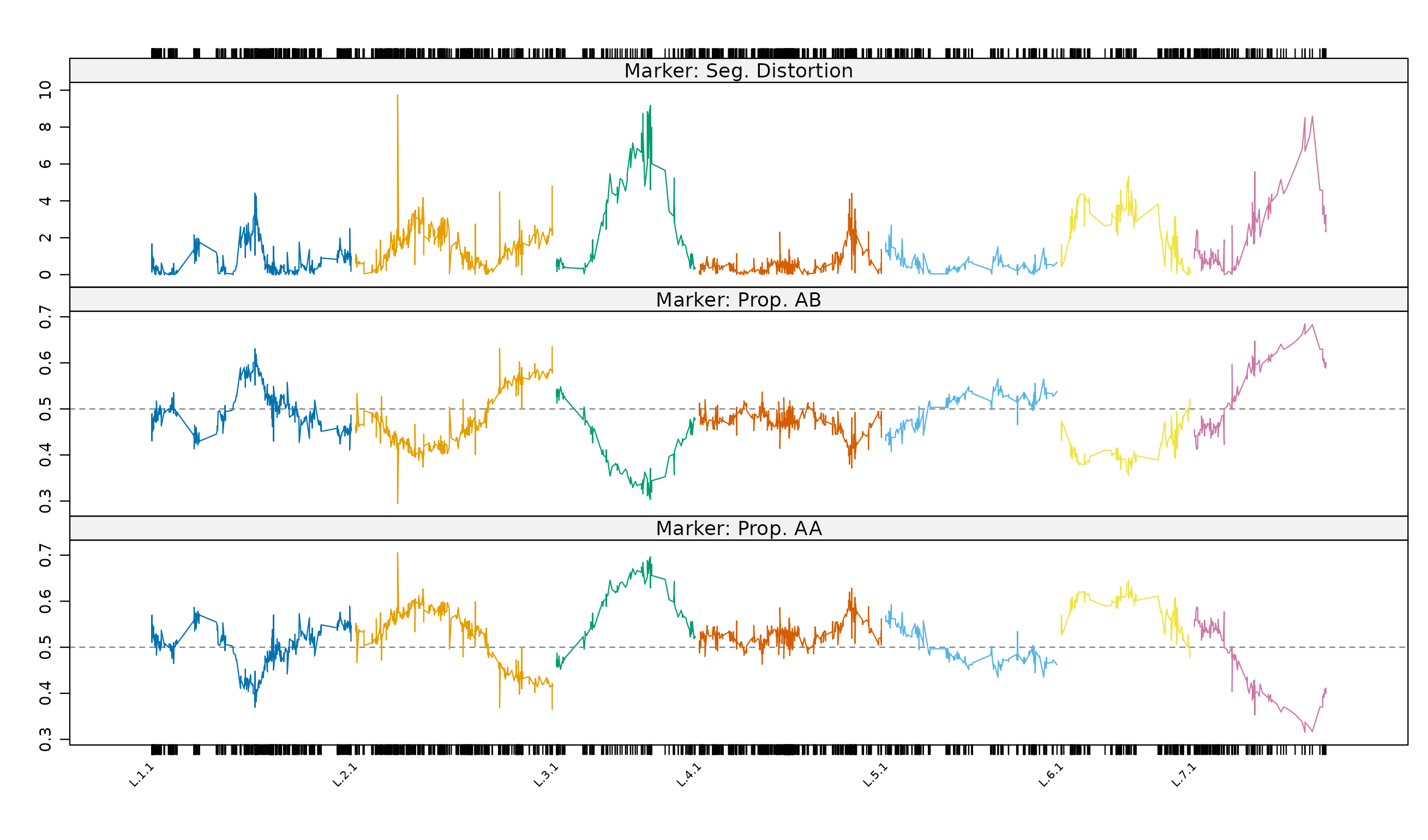

Marker profiles of segregation distortion and allele proportions for mapBC9.

Marker profiles of the negative log10 p-value for the test of segregation distortion and the allele proportions for mapBC9.

A spike of segregation distortion appears on L.2 which does not appear to be biological in origin and should be removed. Significant distortion is also apparent on L.3, L.6 and L.7, indicating that some of the markers with 10 to 20% missing values restored earlier carry a degree of distortion themselves. The marker positions on the horizontal axis suggest these regions are sparse. The 295 markers held in the "seg.distortion" element may account for that sparsity, and are restored to establish their effect.

dm <- markernames(mapBC9, "L.2")[statMark(mapBC9, chr = "L.2",
                                          stat.type = "marker")$marker$neglog10P > 6]
mapBC10 <- drop.markers(mapBC9, dm)
mapBC11 <- pushCross(mapBC10, type = "seg.distortion",
                     pars = list(seg.ratio = "70:30"))
mapBC12 <- mstmap(mapBC11, bychr = TRUE, trace = FALSE, dist.fun = "kosambi",
                  p.value = 2)

Number of linkage groups: 1
The size of the linkage groups are: 680 
The number of bins in each linkage group: 192   
Number of linkage groups: 1
The size of the linkage groups are: 570 
The number of bins in each linkage group: 210   
Number of linkage groups: 1
The size of the linkage groups are: 328 
The number of bins in each linkage group: 93    
Number of linkage groups: 1
The size of the linkage groups are: 673 
The number of bins in each linkage group: 203   
Number of linkage groups: 1
The size of the linkage groups are: 233 
The number of bins in each linkage group: 98    
Number of linkage groups: 1
The size of the linkage groups are: 278 
The number of bins in each linkage group: 97    
Number of linkage groups: 1
The size of the linkage groups are: 218 
The number of bins in each linkage group: 98

round(chrlen(mapBC12) - chrlen(mapBC9), 5)

     L.1      L.2      L.3      L.4      L.5      L.6      L.7 
 0.20398  1.11431  0.60228 -0.92150  0.86448 -0.25043 -6.29943

nmar(mapBC12) - nmar(mapBC10)

L.1 L.2 L.3 L.4 L.5 L.6 L.7 
  0   1 156   0   0  86  52

A distortion ratio of 70:30 was chosen, after inspection of the table held in the "seg.distortion" element, to ensure that all markers were restored. The linkage group lengths change only negligibly from the previous map with the distorted markers removed, which indicates that the additional markers have been inserted successfully, nearly all of them into L.3, L.6 and L.7.

Finally the 39 co-locating markers held in the "co.located" element are restored, each placed adjacent to the marker it co-locates with. Markers of this type carry an immediate linkage group assignment.

mapBC <- pushCross(mapBC12, type = "co.located")
names(mapBC)

[1] "geno"  "pheno"

The additional elements have been removed from the object, leaving only "pheno" and "geno". The final map has the following structure.

	L.1	L.2	L.3	L.4	L.5	L.6	L.7	Total	Average
Number of markers	681	593	335	679	233	279	219	3019	431
Length (cM)	225.9	224.4	157.6	205.5	195.1	145.5	142.9	1297.2	185.3
Average interval (cM)	0.33	0.39	0.48	0.31	0.84	0.53	0.66		0.51

Post-construction development

It is common to develop a linkage map further by inserting additional markers. This may be a straightforward fine mapping exercise, in which the linkage group of the additional markers is known in advance, or a more involved task such as inserting markers from an older map into a newly constructed one.

Either can be problematic. External manipulation, such as the removal of non-concurrent genotypes, may be required before insertion, and the map may need partial or complete reconstruction afterwards. An unfortunate consequence of reconstruction is the potential loss of known linkage group identities.

ASMap allows additional markers to be inserted while preserving those identities. The methods below assume that the additional markers and the constructed map are R/qtl cross objects of the same class. In each example the additional markers are obtained by sampling from the final map, mapBC.

set.seed(123)
add1 <- drop.markers(mapBC, markernames(mapBC)[sample(1:3019, 2700, replace = FALSE)])
mapBCs <- drop.markers(mapBC, markernames(add1))
add3 <- add2 <- add1
add2 <- subset(add2, chr = "L.1")
add3$geno[[1]]$data <- pull.geno(add1)
add3$geno[[1]]$map <- 1:ncol(add3$geno[[1]]$data)
names(add3$geno[[1]]$map) <- markernames(add1)
names(add3$geno)[1] <- "ALL"
add3 <- subset(add3, chr = "ALL")

Combining two maps of the same population

Populations are frequently genotyped on more than one platform, with separate maps constructed from each. A map built from an Illumina 90K SNP array, for instance, may coexist with a legacy map built from SSR or DArT markers. The add1 object mimics such an older map of mapBC, with 319 markers spanning the seven linkage groups. Since the linkage groups are known in both maps, it remains only to combine them sensibly and reconstruct.

add1 <- subset(add1, ind = 2:300)
full1 <- combineMap(mapBCs, add1, keep.all = TRUE)
full1 <- mstmap(full1, bychr = TRUE, trace = FALSE, anchor = TRUE, p.value = 2)

Number of linkage groups: 1
The size of the linkage groups are: 681 
The number of bins in each linkage group: 192   
Number of linkage groups: 1
The size of the linkage groups are: 593 
The number of bins in each linkage group: 209   
Number of linkage groups: 1
The size of the linkage groups are: 335 
The number of bins in each linkage group: 93    
Number of linkage groups: 1
The size of the linkage groups are: 679 
The number of bins in each linkage group: 202   
Number of linkage groups: 1
The size of the linkage groups are: 233 
The number of bins in each linkage group: 99    
Number of linkage groups: 1
The size of the linkage groups are: 279 
The number of bins in each linkage group: 97    
Number of linkage groups: 1
The size of the linkage groups are: 219 
The number of bins in each linkage group: 98

This is a characteristic application of combineMap(), described in Manipulating linkage maps. The maps are first merged on their matching genotypes; because the first genotype of add1 has been removed, missing cells are inserted in the first genotype of mapBCs for the markers contributed by add1. The function recognises that both maps share linkage group names and places the markers from shared groups together. Reconstruction by linkage group with p.value = 2 then retains those identities, and anchor = TRUE preserves the orientation of the larger map.

Fine mapping

In marker assisted selection it is common to increase marker density in a specific genomic region, so that the position of quantitative trait loci may be identified more accurately. The add2 object contains markers from the L.1 group of mapBCs alone. Where the linkage group of the additional markers is known in advance and matches a group in the constructed map, insertion proceeds much as above.

add2 <- subset(add2, ind = 2:300)
full2 <- combineMap(mapBCs, add2, keep.all = TRUE)
full2 <- mstmap(full2, chr = "L.1", bychr = TRUE, trace = FALSE, anchor = TRUE,
                p.value = 2)

Number of linkage groups: 1
The size of the linkage groups are: 681 
The number of bins in each linkage group: 192

The removal of the first genotype of add2 again introduces missing values in the first genotype of full2. The reconstruction differs only in that ordering is required within L.1 alone.

Unknown linkage groups

The linkage group of the additional markers is not always known in advance. An incomplete marker set may have been used to construct the map, or a secondary set may be available from an unconstructed map. Here the add3 object consists of a single group named ALL containing all the markers that spanned the seven groups of add1.

add3 <- subset(add3, ind = 2:300)
full3 <- combineMap(mapBCs, add3, keep.all = TRUE)
full3 <- pushCross(full3, type = "unlinked", unlinked.chr = "ALL")
full3 <- mstmap(full3, bychr = TRUE, trace = FALSE, anchor = TRUE, p.value = 2)

Number of linkage groups: 1
The size of the linkage groups are: 681 
The number of bins in each linkage group: 192   
Number of linkage groups: 1
The size of the linkage groups are: 593 
The number of bins in each linkage group: 209   
Number of linkage groups: 1
The size of the linkage groups are: 335 
The number of bins in each linkage group: 93    
Number of linkage groups: 1
The size of the linkage groups are: 679 
The number of bins in each linkage group: 202   
Number of linkage groups: 1
The size of the linkage groups are: 233 
The number of bins in each linkage group: 99    
Number of linkage groups: 1
The size of the linkage groups are: 279 
The number of bins in each linkage group: 97    
Number of linkage groups: 1
The size of the linkage groups are: 219 
The number of bins in each linkage group: 98

combineMap() again merges the maps, avoiding any need to match the dimensions of the marker sets manually. pushCross() with type = "unlinked" and unlinked.chr = "ALL" then distributes the additional markers among the remaining linkage groups of full3, after which ordering within groups is all that is required.

References

Taylor, Julian, and David Butler. 2017. “R Package ASMap: Efficient Genetic Linkage Map Construction and Diagnosis.” Journal of Statistical Software 79 (6): 1–29. https://doi.org/10.18637/jss.v079.i06.