Construction is rarely a single operation. Linkage groups may need to be broken or merged, maps built on different marker platforms may need to be combined, and individuals may need to be removed. The functions described here perform these operations on an R/qtl cross object while preserving the additional structures ASMap places within it.
| Function | Operation |
|---|---|
breakCross() |
Split linkage groups at nominated markers |
mergeCross() |
Combine nominated linkage groups into one |
combineMap() |
Merge separate cross objects into a single map |
subsetCross() |
Subset genotypes or linkage groups consistently |
quickEst() |
Estimate genetic distances rapidly |
Breaking and merging linkage groups
The split argument of breakCross() takes a
list whose elements are named by the linkage groups to be split, and
which contain the markers immediately preceding each
split point. Splitting 3B after its seventh marker and 6A after its
fifteenth is therefore expressed as follows.
mapDHb1 <- breakCross(mapDH, split = list("3B" = "3B.m.7", "6A" = "6A.m.15"))
nmar(mapDHb1)
1A 1B1 1B2 1D 2A 2B 2D1 2D2 3A 3B.1 3B.2 3D 4A 4B 4D 5A
41 5 33 10 40 35 8 13 37 7 23 6 30 32 6 54
5B 5D 6A.1 6A.2 6B 6D 7A 7B 7D
56 6 15 12 41 15 33 37 4 Multiple linkage groups, and multiple split points within a group,
may be handled in a single call. By default a numeric suffix is appended
to the name of the group being split, separated by sep.
Complete names for the new groups may be supplied instead by naming them
explicitly in suffix.
mapDHb2 <- breakCross(mapDH, split = list("3B" = "3B.m.7"),
                      suffix = list("3B" = c("3B1", "3B2")))
nmar(mapDHb2)
1A 1B1 1B2 1D 2A 2B 2D1 2D2 3A 3B1 3B2 3D 4A 4B 4D 5A 5B 5D 6A 6B
41 5 33 10 40 35 8 13 37 7 23 6 30 32 6 54 56 6 27 41
6D 7A 7B 7D
15 33 37 4 mergeCross() performs the converse operation. Its
merge argument takes a list whose elements are named by the
proposed linkage group names and which contain the groups to be
merged.
mapDHm <- mergeCross(mapDHb1, merge = list("3B" = c("3B.1", "3B.2"),
                                           "6A" = c("6A.1", "6A.2")))
nmar(mapDHm)
1A 1B1 1B2 1D 2A 2B 2D1 2D2 3A 3B 3D 4A 4B 4D 5A 5B 5D 6A 6B 6D
41 5 33 10 40 35 8 13 37 30 6 30 32 6 54 56 6 27 41 15
7A 7B 7D
33 37 4
mergeCross()inserts an artificial genetic distance gap between the merged groups, governed by thegapargument. The distances across the join are therefore not estimates, and a separate estimation step is required after merging.
Combining maps
A recurring requirement in linkage map construction is the merging of
cross objects, for instance where two maps of the same population have
been built independently from markers on different platforms.
combineMap() addresses this, merging maps on the basis of
their map information so that the combined linkage groups are ready for
reconstruction by mstmap.cross().
Any number of maps may be supplied. They must share the same cross
class structure and the same genotype identifier id, and
marker names must be unique across all of the maps supplied.
Merging proceeds in two stages. Maps are first merged on the
genotypes they have in common: with keep.all = TRUE the
combined map is padded with missing values where genotypes are not
shared, whereas with keep.all = FALSE it is reduced to
those genotypes common to every map. Linkage groups bearing the same
name across maps are then merged, and groups whose names are not shared
are retained separately.
The example below duplicates mapDH, renames ten of its
linkage groups and alters the marker names within each group to ensure
uniqueness.
mapDH1 <- mapDH
names(mapDH1$geno)[5:14] <- paste("L", 1:10, sep = "")
mapDH1$geno <- lapply(mapDH1$geno, function(el) {
  names(el$map) <- dimnames(el$data)[[2]] <- paste(names(el$map), "A", sep = "")
  el
})
mapDHc <- combineMap(mapDH, mapDH1)
nmar(mapDHc)
1A 1B1 1B2 1D 2A 2B 2D1 2D2 3A 3B 3D 4A 4B 4D 5A 5B 5D 6A 6B 6D
82 10 66 20 40 35 8 13 37 30 6 30 32 6 108 112 12 54 82 30
7A 7B 7D L1 L2 L3 L4 L5 L6 L7 L8 L9 L10
66 74 8 40 35 8 13 37 30 6 30 32 6 The combined map holds a merged marker set for those linkage groups that shared a name, and distinct groups for those that did not.
combineMap()merges maps but does not reconstruct the result, and it applies no consensus map algorithm. Chromosome identity and genetic distances are taken from the first appearance of a marker across the maps supplied. Runmstmap()afterwards.
The value of combining before reconstructing is not immediately obvious. Reconstructing the union of several maps directly would discard the identity of the linkage groups; combining first preserves it. Applications of this in practice are given in Worked example II.
Subsetting
pullCross() and pushCross() create the
additional list elements "co.located",
"seg.distortion" and "missing", each holding a
marker matrix whose row dimension matches the marker elements of the map
it was drawn from. These elements are not known to R/qtl.
Using
subset.cross()on an object carrying those elements will subset the map but not the elements within it. Their data components will retain the removed individuals, and the statistics in the tables of the"seg.distortion"and"missing"elements will no longer describe the map. Nothing reports this.
subsetCross() provides the functionality of
subset.cross() while subsetting those data components to
match, and additionally recalculates the table components of the
"seg.distortion" and "missing" elements. That
recalculation matters, because pushCross() consults those
statistics when deciding which markers to restore.
mapDH.s <- pullCross(mapDH, type = "seg.distortion")
mapDH.s <- subsetCross(mapDH.s, ind = 3:218)
dim(mapDH.s$seg.distortion$data)[1]
[1] 216The data component of the "seg.distortion" element now
has the same dimension as the map.
Rapid genetic distance estimation
The map estimation function of R/qtl, est.map(), applies
the multi-locus hidden Markov model of Lander and
Green (1987). That approach is
computationally demanding for linkage groups carrying many markers, and
increasingly so in the presence of missing allele calls and genotyping
errors.
quickEst() circumvents this by a different route. It
calls argmax.geno() from R/qtl, itself a multi-locus hidden
Markov algorithm, but requires reconstruction only at the markers
themselves rather than at imputed pseudo-markers. Accurate imputation
requires an initial estimate of genetic distance, which is obtained by
calling est.rf() within each linkage group nominated by
chr and converting the recombination fractions to distances
according to map.function.
map1 <- est.map(mapDH, map.function = "kosambi")
map1 <- subset(map1, chr = names(nmar(map1))[6:15])
map2 <- quickEst(mapDH, map.function = "kosambi")
map2 <- subset(map2, chr = names(nmar(map2))[6:15])
plotMap(map1, map2)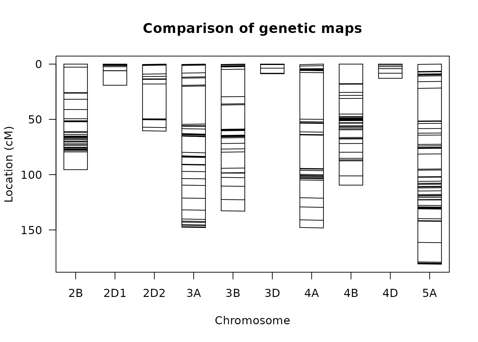
Comparison of mapDH estimated using est.map()
and using quickEst().
The comparison shows negligible differences in marker placement and in overall linkage group distances between the two methods.
Further reading
-
Pulling and pushing markers —
the elements that make
subsetCross()necessary - Worked example II — merging linkage groups and combining maps in practice
- Constructing a linkage map — reconstruction after any of these operations